Usage
Using RadioViz is very simple and very intuitive. Just follow your flow to get the things done.
Start the program
From any console, type radioviz to start the program. The main window will show up in a few seconds.
Open autoradiography images
The tool is meant to open TIFF and XYZ files. Any attempt to open different formats is rejected. Typically autoradiography images are gray-scale, if you try to open an RGB file, this will be converted to Gray-scale but results might be unpredictable.
To open one or more file, follow the File > Open… to obtain a file selection dialog where you can select one or more TIFF or XYZ files.
You can also use the File > Open Recent menu to recall one of the five last opened images.
Alternatively you can drag-and-drop the TIFF or XYZ files you want to open directly on the RadioViz main window to open them.
XYZ files produced by the scanner typically have a matching .dat sidecar file with the same name. The DAT file contains acquisition metadata that RadioViz uses to populate the TIFF tags when saving derived images. When a DAT file is missing, RadioViz prompts you to select one or continue without metadata. You can still save XYZ files as TIFF, but the resulting metadata will be incomplete if no DAT is provided.
If a DAT file reports image dimensions that do not match the actual XYZ data, RadioViz preserves the image size from the XYZ file and shows a warning. Saving as XYZ does not generate a DAT sidecar; RadioViz will show a warning to remind you that metadata will not be preserved unless you create the DAT file separately.
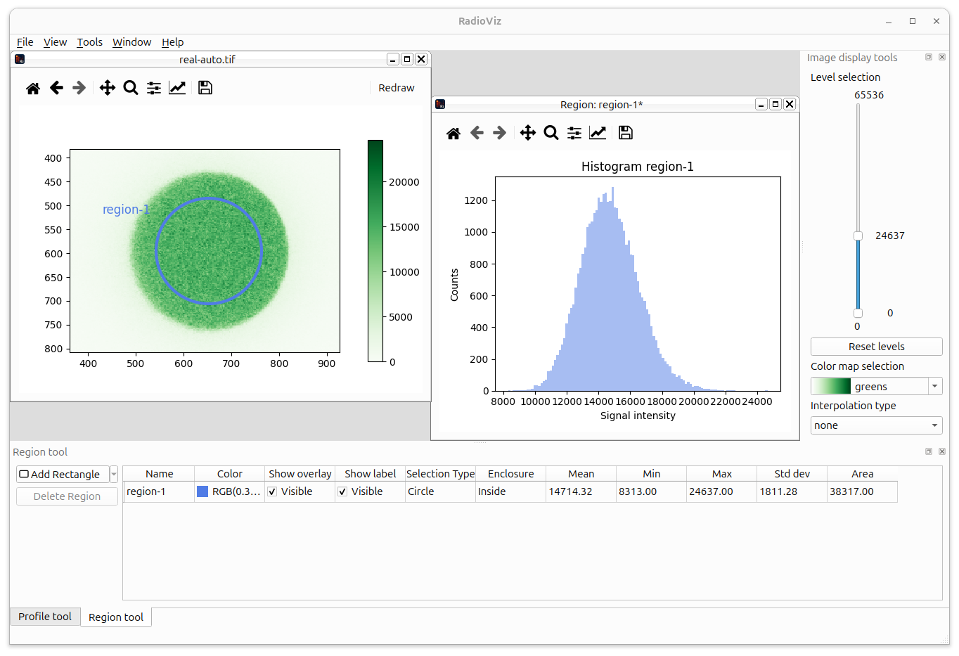
The opened images will be displayed with the default settings as in the image here below:
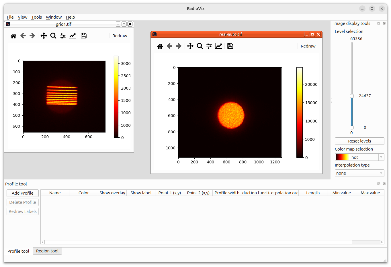
Each of the images is represented in a Matplotlib Canvas with its colorbar on the right hand side. The canvas has also the standard navigation toolbar to pan / zoom the image.
When moving the mouse over the image, the x, y coordinates and the signal intensity will be displayed on the right hand side of the navigation bar.
Clicking on the Floppy Disk icon, you can save an image file of the current visualization. Very handy for preparing presentation images.
When a large image is opened, a downscaled version is displayed because it makes no sense to show an image with more pixels than the screen can actually display. Zooming in will trigger the display of a finer image up to the full resolution.
Playing with levels and other visualization parameters
As mentioned before, autoradiography images are grayscale, but nevertheless it is very practical to use a different color map or to change the visualization levels to underlying a feature.
For this purpose, one can use the Image display tools docking window. The docking window has two tabs: Levels and Scale. From the Levels tab, simply play with the range slider to select the minimum and maximum value to display. If you want to set a specific value for them, you can double click on the cursor label and you will be allowed to enter the desired value.
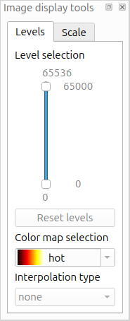
By default, the image is displayed with the whole range, assuming a 16-bit dynamic range. If you want to restore the initial range, click on the Reset Levels button.
You can choose among a list of different color maps from the drop down combobox. Similarly, you can change the interpolation algorithm used to display the images. The default mode is none.
Axis labels and scale bars
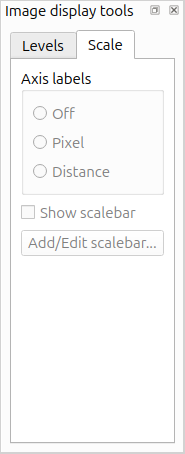
Switching to the Scale tab, you can set axis labels and scale bars. Use the axis label radio buttons to switch between:
Off (hide axes)
Pixel (show pixel numbers)
Distance (show real distances computed from the image metadata)
If a valid pixel size is available, you can enable the scale bar with Show scalebar and fine‑tune it with Add/Edit scalebar…. The dialog lets you control bar length/height and its colors.
You can also modify both axis labels and the scale bar from the context menu: Display > Axis labels and Display > Scalebar.
Workspaces
A workspace is a snapshot of an ongoing analysis. It stores the opened images, display parameters, tool state, overlays, and any other data needed to restore the session later. This is useful when you want to pause an analysis and resume it later without repeating the setup steps.
RadioViz supports two workspace formats:
JSON workspace (.json): Human-readable and easy to inspect or version-control. Best for small-to-medium workspaces and for debugging or manual tweaks. The downside is that data are not stored inside the workspace dump, so, for example, in the case of image window, the JSON file will contain only the path to the original image. If the file is deleted from disc or moved, the restore of the JSON workspace will fail. Analysis results, like profiles and histograms, are not saved, but recalculated starting from the original information.
HDF5 workspace (.h5): Efficient for large numeric data and generally faster for big sessions. It is compact and optimized for arrays, but it is not human-readable and is less convenient for manual inspection or diffing. Everything is saved in the HDF file, including the image and the analysis data. A HDF5 workspace can always be restored even if the original images are deleted / moved because it is actually embedding a copy of them.
In short, choose JSON to obtain a very lightweight, human-readable, version-control friendly format. All analysis steps will be repeated while the workspace is restored. Choose HDF5 if you want to be sure that everything is saved, it will take a bit of disc space, but the restore will be super fast.
Analysing intensity profiles
Extracting an intensity profile from a 2D image is very relevant for autoradiography experiments.
To do so, the user can rely on the Profile tool docking window.
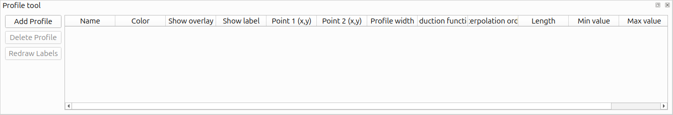
This window is composed by a table containing a list of all the already existing profiles and three buttons to create and delete a new profile respectively and redraw all labels.
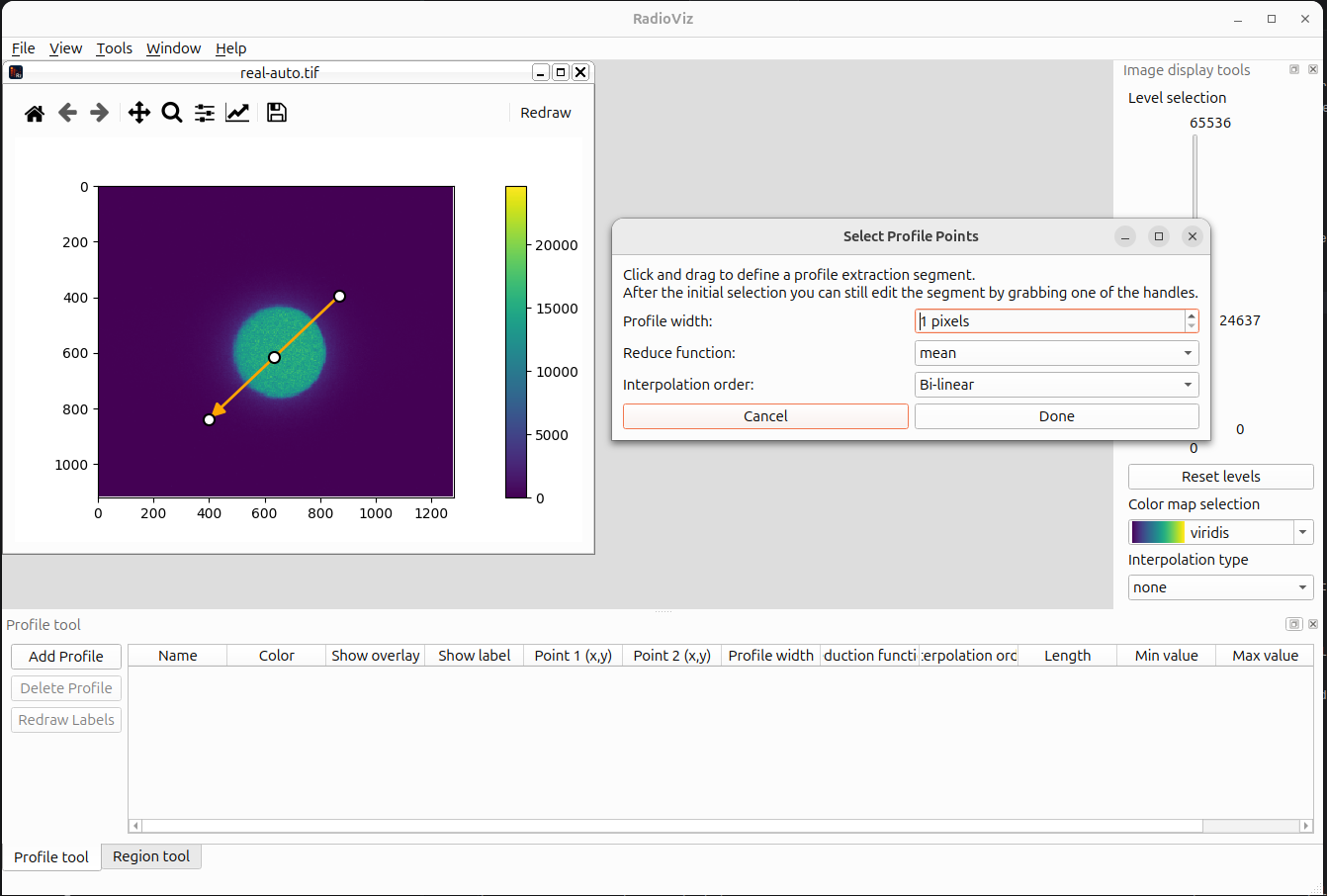
To add a new profile, you need to have opened a TIFF image and having selected it. Then click on Tools > Analysis > Profile > Add Profile to start the profile definition procedure. A dialog window will appear where you can select the width in pixel of the profile, the reduce function to be used in case of width greater than 1 and the interpolation order. You can then start drawing the profile path by clicking and dragging the mouse on the image. A temporary arrow is drawn and you can still edit the start, the end and the overall position by clicking and dragging the corresponding arrow handles. The profile is calculated only when you click the done button of the dialog window.
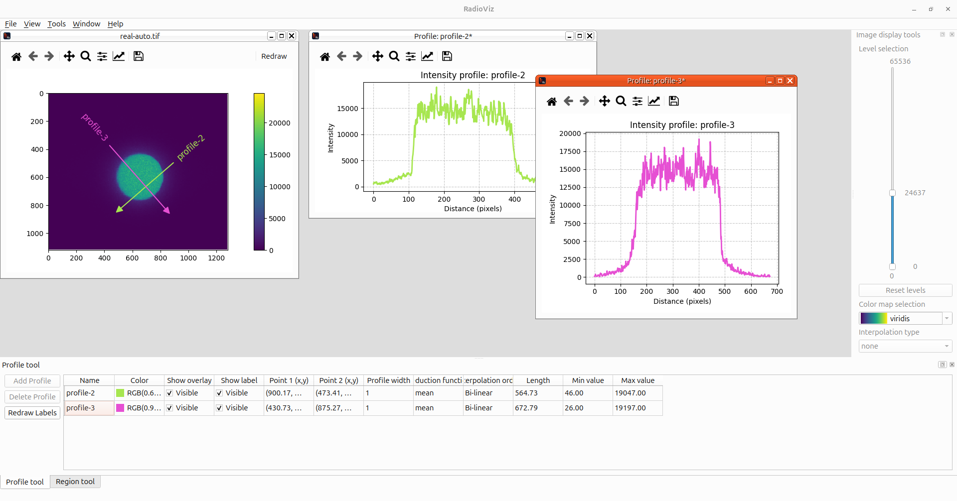
After clicking on the done button, the intensity profile is extracted according to the specified parameters and a new window is opened to display the output. The original autoradiography image gets a persistence arrow overlay with the name of the profile and a unique color. From the table view in the Profile tool docking widget is possible to select one specific profile, change its name, the visibility of the arrow and of the label.
You can remove existing profiles, selecting them in the table and clicking on Delete Profile button.
If spatial calibration metadata are available, the profile window can display the distance axis in real units. Right‑click inside the profile window and use Display > Axis labels > Pixel/Distance to switch between pixel and calibrated units. The profile tool table includes both the pixel length and a calibrated length column (value + unit) so you can quickly compare profiles with different units.
Analysing areas
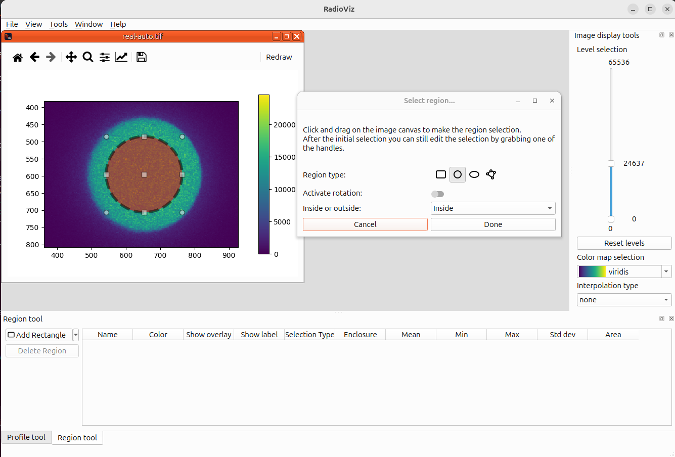
Along with 1D analysis, you can also obtain 2D information with the Region Tool. The region dock widget is similar to the profile one, with a multi-button to add an area with different geometry (rectangle, circle, ellipse and polygon), another button for removing the selected region and a table with the list of all existing region analysis. The add region button becomes active when an autoradiography image is activated. Clicking the button will start the interactive region definition procedure guided by a dialog window where you can change the region type, activate the possibility to rotate the selection (only for rectangle and ellipse) and a selector to decide if you are interested in the inside or outside of the selection. You can start the region selection procedure also from the Tools menu.
The region definition is done very intuitively with mouse click and drag on the image. A temporary selection is shown and can be adjusted by dragging the various handles. In the case of a polygonal selection, click on the first point and then add as many points as you like before closing the region by clicking again on the first point.
Once you are happy with the selection, click done on the dialog window to start the region analysis calculation. When ready, a new windows will appear containing the frequency histogram of the pixel signal.
Measuring distances and angles
RadioViz provides a Measurement Tool to measure segment lengths and angle amplitudes directly on image windows. The measurement dock includes two tables (segments and angles) plus a single add menu button.
To create a segment measurement, select an image window and click Tools > Analysis > Measure > Segment or use the Add Measurement button in the dock. A dialog will guide you to click and drag a line on the image. Once the selector is visible, you can adjust it by dragging the handles. Press Done to accept and create the measurement overlay.
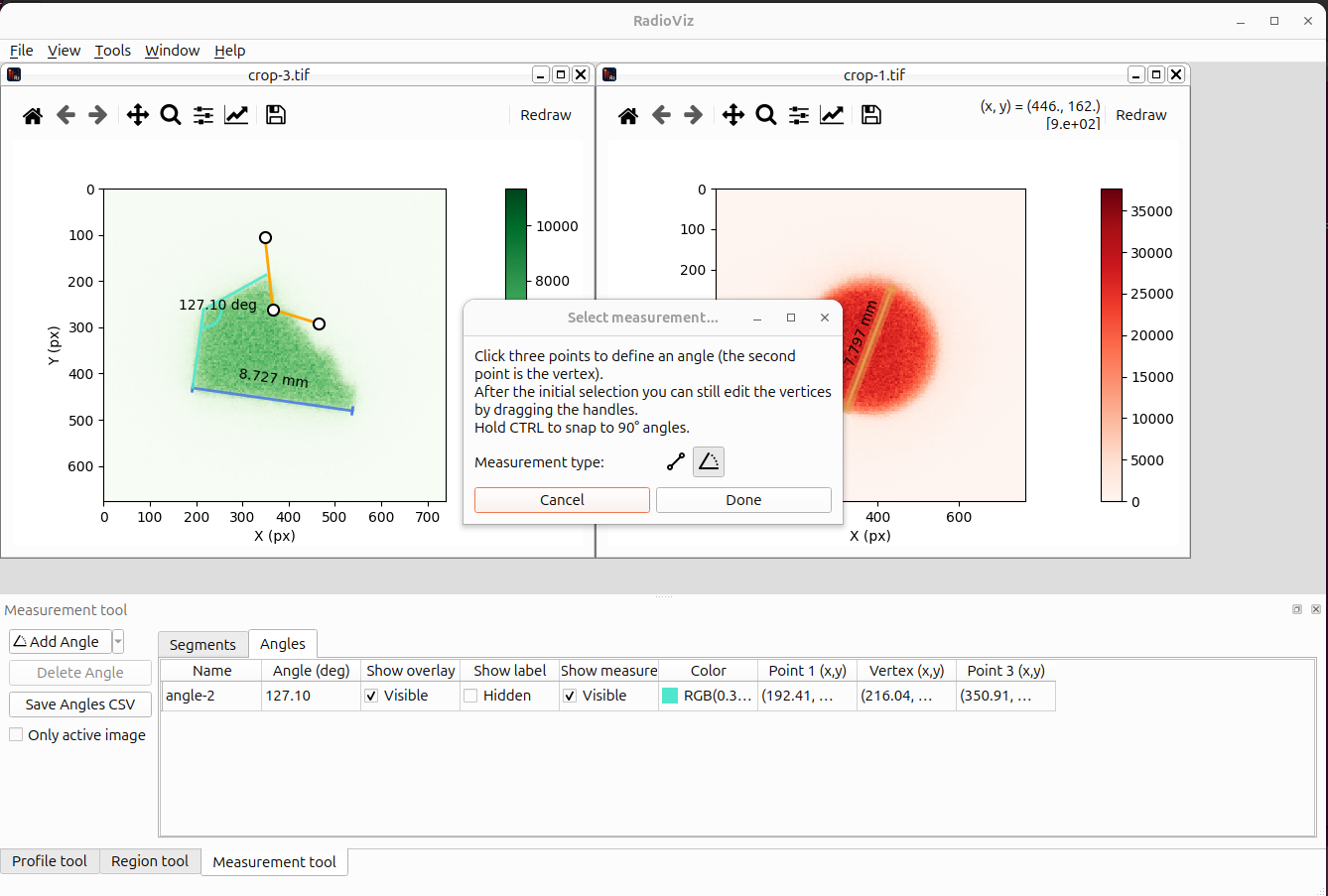
To create an angle measurement, select Tools > Analysis > Measure > Angle. Click three points on the image (the second point is the vertex of the angle). You can still edit the points before confirming the selection.
The segment table shows both pixel length and calibrated length (when spatial calibration metadata are available). The angle table shows the measured angle in degrees. Each table row lets you rename the measurement, toggle the overlay visibility, show/hide labels, and show/hide the measurement value. The dock also provides buttons to export each table to CSV and a checkbox to filter items to the active image only.
Note
When selecting the three points to build an angle, you are actually drawing two intercepting segments. From a geometrical point of view, this is defining two angles whose sum is 360°. RadioViz will always provide the value of the smallest of the two and assume that the user can calculate the other one, if needed, by difference.
Flipping images (horizontal or vertical)
RadioViz can flip the active image horizontally or vertically without resampling. The flip can create a new image window or update the current image in-place.
To flip an image, select it and choose one of the following menu entries:
Tools > Transform > Horizontal flip > New image…
Tools > Transform > Horizontal flip > In place…
Tools > Transform > Vertical flip > New image…
Tools > Transform > Vertical flip > In place…
If you select in-place output and dependent analyses exist, RadioViz warns you and asks for confirmation because those dependent items become invalid and are removed.
Aligning images to a reference line
The Align image tool rotates an image so that a user-defined line becomes horizontal or vertical.
To start, select an image and click Tools > Transform > Align image to line…. A dialog opens where you can choose:
target alignment (horizontal or vertical)
output mode (new image window or in-place)
interpolation order
image extension policy - fill with a constant value (default 0) - crop to the largest valid rectangle (no synthetic fill pixels)
While the dialog is open, draw and edit the line directly on the image canvas. Click OK to run the rotation. The calculation runs in a background thread to keep the UI responsive.
If you choose in-place output and dependent analyses exist (for example profiles or regions), RadioViz warns you and asks for confirmation because those dependent items become invalid and are removed.
Autocropping regions
The Autocrop tool allows you to automatically detect and crop regions of interest in autoradiography images. This tool uses Otsu’s thresholding algorithm combined with region labeling to identify areas of interest in images.
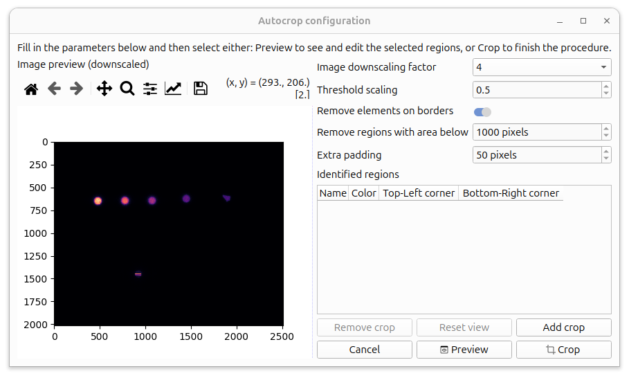
To use the autocrop tool, select the Tools > Crop > Autocrop menu. This will open a configuration dialog where you can adjust the following parameters:
Image downscaling factor: Controls the level of image downscaling for faster processing. Options are 1x, 2x, 4x, 8x, and 16x.
Threshold scaling: Multiplier for the Otsu threshold value used for binary conversion. Values range from 0.1 to 1.0.
Remove elements on borders: Toggle to remove regions touching the image borders.
Remove regions with area below: Minimum area threshold for regions to be considered (in pixels).
Extra padding: Additional padding to add around detected regions (in pixels).
After setting the parameters, click Preview to visualize the detected regions. You can then select individual regions in the table view and adjust their positions by dragging the edges of the rectangles. When you select an item in the table, the canvas containing the whole image will be redraw to show a zoomed-in range around the selected item. If you want to restore the full view, just click the Reset view button.
To add custom regions, click the Add crop button to enter manual selection mode. Draw a rectangle on the image to define a custom crop region.
Cropped areas are numbered row-wise from left to right. They can be renamed by editing their label in the table view. The label name will be used as the name for the new image.
When you’re satisfied with the regions, click Crop to perform the actual cropping. The tool will create new image windows for each cropped region, preserving the original image metadata and derivation information.
After cropping regions, you can visualize the crop areas on the original image by using the Show/Hide ROI on original image option from the Autocrop menu. This feature displays a dashed rectangle overlay with a label indicating the crop region on the original image. You can toggle the visibility of these overlays using the same menu option. This is particularly useful for verifying that the cropping regions correspond to the intended areas of interest in your original image.
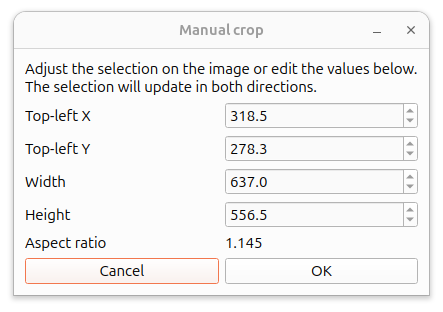
Manual cropping
If the autocropping functionality does not work for you or if you have an image configuration where a manual user decided cropping tools is more suitable, instead of selecting Autocrop, just use the Manual crop. The tool will allow you to select a rectangular region on the currently selected image. The cropping selection can be edited either by acting directly on the selector handle on the image or by entering values in the dialog window below for the coordinates of the top left corner and the width and height of the selection. The aspect ratio is kept updated for your convenience.